STARK: FRI with concrete numbers for software engineers

Introduction

In this article, I’ll walk you through the FRI protocol, which is central to zkSTARK for great efficiency, through concrete numbers. If you’re one who’s interested in STARK and FRI, you must have heard and known a bit about FRI. There are already some great blog posts (StartWare’s post and Vitalik’s post) and working codes (Distaff and RISC Zero) worth looking at. However, despite the presence of these resources, I felt I was not somewhat getting some pieces of FRI as a software engineer, not a cryptographist. That’s why I decided to write up this article full of concrete (but of course in a finite field) numbers for a more clear explanation. I’m a bit confident that, if you’re an ordinary software engineer like me, this article helps you to figure out how and why the FRI protocol works. A bit more about my explanation strategy, I’ll start with a strawman solution that keeps the core concept of FRI but omits some details and get a solution better step by step.

PS: all the examples used throughout this article can be found in this repo as working codes.

The aim of FRI

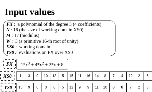
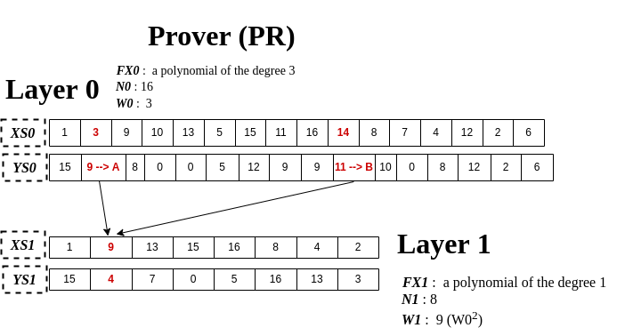
First of all, I’ll give you a set of concrete numbers used throughout this article. There is a polynomial, FX, of degree 3. And we have a set of points that are on FX. Its domain, XS0, is generated by the above finite field configuration (see N, M, W). YS0 is a set of evaluations of FX over XS0. (i.e., FX(1)=15, FX(3)=9, …)

In this configuration, say that there are two actors, Prover (shortly PR) and Verifier (shortly VR). And PR wants to prove to VR that YS0 is a set of evaluations that are on a polynomial of degree 3, no matter what the coefficients of FX are. To do so, PR just sends YS0 to VR, and VR verifies whether it’s of degree 3.

Here, the straightforward way for VR to verify it is to pick arbitrary 4 points to interpolate FX (of degree 3) again and check if all other points are on the computed FX. If any point changes, this verification will fail. But this method is somewhat inefficient as it incurs linearly increasing overheads, which means if N gets much larger, both interpolation and verification overheads will increase accordingly. This is where FRI comes into play.

The aim of FRI is to allow VR to verify the same thing more efficiently with the aid of PR. The method to do it is as follows in a nutshell.

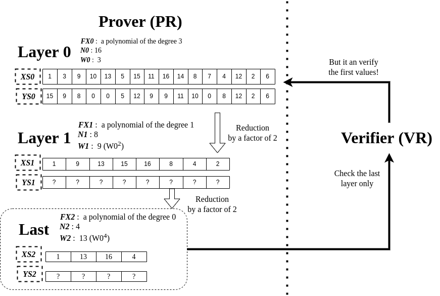
The key idea is called low-degree testing, which reduces by a factor of 2 (it can also be 4 or 8) the size of evaluations (YS0) to check on the VR side. In other words, if Layer 1 is the last layer, it’s enough for VR to interpolate any 2 points of YS1 (since FX1 is of degree 1) and check the rest 6 points, which is half overhead compared to checking YS0. The point here is that VR checks much smaller points (YS1 or YS2) than the original points (YS0) but still can guarantee YS0 (original data) is of degree 3. This is why it’s called low-degree testing because it allows testing a polynomial at a lower degree. What’s more, this reduction technique can be applied recursively until FXn reaches a degree 0. (when to stop this reduction is configurable) OK, then, what makes this low-degree testing get possible? What does this reduction exactly look like? I’ll talk about this in the following.

A reduction technique

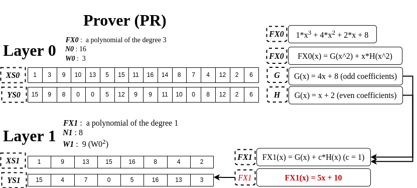
On the PR side, a degree reduction technique by a factor of 2 is illustrated in the above picture. FX0 is what we’re targeting to reduce a degree. First, we can rewrite FX0(x) by introducing the two new functions, G and H, FX0(x) = G(x^2) + x*H(x^2), and set the odd/even coefficients of FX0 to G and H, respectively. And then, it will lead to FX1 which is used in the next layer. It’s worth noting that FX1 has c, but for now, we set 1 to it, but remember this c as it will come in handy later.

Once all of YS1 is computed, PR makes a verification request to VR including YS0 and YS1. Afterward, VR starts trying to verify it. Since YS0 and YS1 are the only things VR can get (FX0 is not sent), VR has to be capable of computing YS1 by using YS0.

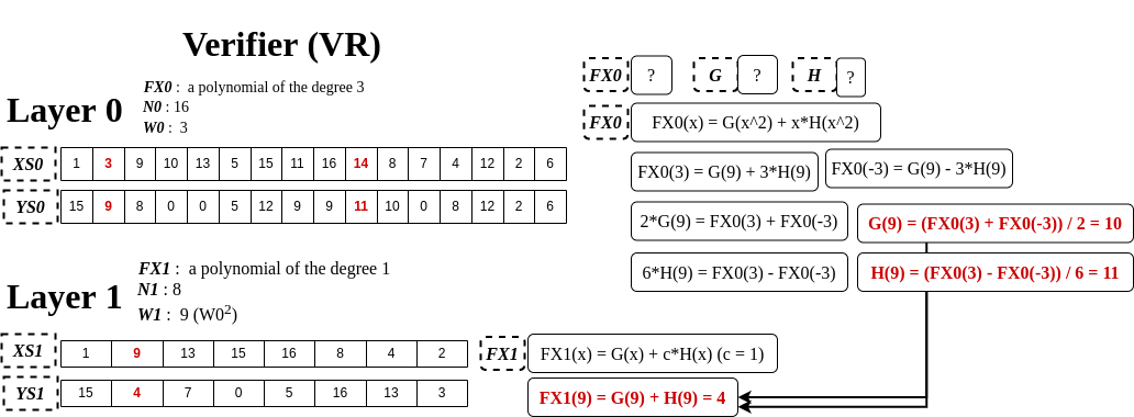
The above picture depicts how VR computes an element, FX1(9). As you can see, to solve FX1(9), we need to know G(9) and H(9). To do so, we first take two x values where x^2=9. They are 3 and -3 (-3 is equal to 14 in this finite field). And with FX0(3) and FX0(-3), it’s able to compute G(9) and H(9), as illustrated on the right side of the picture. Same way, we can compute all YS1 values without having to know what FX0 is. Once VR determines YS1, at this point what VR has is (YS0, YS1 (PR sent)) and (Computed_YS1) where Computed_YS1 is what’s computed by VR, not sent by PR. Then, finally, VR can start verification as follows.

1. Layer value check- Check if Computed_YS1 == YS1. If not matched, PR is a possibly malicious prover.

2. Last layer degree check- If Layer 1 is the last layer, check whether YS1 is on a polynomial of degree 1. If not, PR is a possibly malicious prover. (If Layer 1 is not the last one, try computing YS2 and verifying the same way)

Only when these two checks pass, VR believes that PR is a genuine prover and YS0 is indeed on a polynomial of degree 3. To see if it can actually detect an attack, take a simple modification of XS0, getting FX0 a different degree than 3. When we change FX0(3) = 9 → 10, it gets FX1(9) = 7, which means any modification of YS0 affects YS1 where the final verification takes place. So, it will result in the violation of the second verification check.

Ok, then, is this system perfect regarding security? Absolutely not. There’s still room for a malicious prover to cheat a verifier. I’ll talk about it in the following section.

A successful attack and an interactive proof

I want to first define what cheating a verifier means in this protocol. If FX1 (say Layer 1 is the last one) turns out to be of degree 1 (or any target degree) even when FX0 is not on degree 3, it can be called a successful attack. For a more visualized explanation, see below.

Imagine that a malicious prover (shortly MPR) carefully picks values for FX0(3) and FX0(-3) that affect FX1(9). I mean, MPR obviously changes (1) from FX0(3) to A, (2) from FX0(-3) to B, but this combination of A and B leads to the same FX1(9)=4. In spite of this attack, VR gets to trust PR because YS1 is actually of degree 1. MPR can simply do brute-force to find out proper A and B. (An example for A and B is 1 and 10)

By now, you may get how easy it is to cheat a verifier here. Then, how can we stop this attack? The key to it is c in FX1(x)=G(x) + c*H(x). Let’s think about why this attack can happen. That’s because MPR can correctly compute FX1(x) as c is 1. How about generating a random challenge c on the VR side and sending it to PR, like below?

1. [PR] Send YS0 to VR.

2. [VR] Generate a random challenge c and send it to PR.

3. [PR] Compute YS1 using the given c and send YS1 to VR.

4. [VR] Verify.

See how the aforementioned attack gets blocked in the above interactive scheme. In Step 1, PR can’t compute YS1 because c is not determined yet. So, the only thing PR can do is make a random guess on c and compute YS1 accordingly. However, it will fail with a high probability. Ok, we’ve got to this point where cheating can be prevented through an interactive proof system. But, this system incurs considerable communication overheads between PR and VR, as it demands more communication as N increases for Layer N. Then, what we should do next is turn this system into a non-interactive system while not sacrificing security.

Turns into a non-interactive proof

We’re going to use the Fiat-Shamir heuristic to turn it into a non-interactive system. In a nutshell, this technique is about replacing the use of random challenge with the use of a cryptographic hash function.

1. [PR] c1 = Hash(YS0)

2. [PR] Compute YS1 using the computed c1.

3. [PR] send YS0 and YS1 to VR.

4. [VR] c2 = Hash(YS0)

5. [VR] Compute Computed_YS1 using c2 and verify it.

In the use of Hash(YS0) for a random challenge (generally speaking, we have to put YS0, which directly relates to a proof statement, in a hash function), PR can’t make a correct guess on YS1. This is because corrupting YS0 negates all of YS1 built on top of c1.

Thus far, we’ve built a non-interactive secure proof system in which there’s no necessary communication. We call, a set of data needed to be passed on from PR to VR, FRI proof, which contains YS0 and YS1. However, there is one more inefficiency left here. That is, when N gets too large, the size of FRI proof gets huge accordingly and “Layer value check” turns to a large overhead. We’ll move on to how to reduce these inefficiencies down to a constant level or a log level.

A configurable number of query

The key idea to get the size of FRI proof manageable (“Layer value check” overhead as well), is to limit the number of checks to a constant. Let’s take one additional variable, named NUM_QUERY, which literally means how many times it would check and is configurable. And say NUM_QUERY = 2 and where to check is {0, 2} that we call QUERY_POSITION.

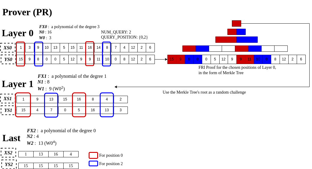
This combination of NUM_QUERY and QUERY_POSITION means, in this concrete context, VR has to check if YS1[0] and YS1[2] match (i.e., 15 and 7). In order for VR to compute YS1[0], PR has to give YS0[0] and YS0[8] (in red boxes), and for YS1[2] it has to have YS0[2] and YS2[10] (in blue boxes). That is, PR has to send NUM_QUERY*2 elements to VR for each layer except the last one. For the last layer, all YS2 have to be given for “Last layer degree check”. (PS. precisely, NUM_QUERY*2 is the maximum of what needs to pass)

But, there’s one practical issue arising. That is, VR needs to know all of YS0 in order to get the random challenge to compute YS1 correctly. If PR just sends chosen values of YS0, VR cannot retrieve the random challenge, leading to a false alarm. This protocol adopts the Merkle Tree, as a means of delivery, to solve this problem. In other words, PR provides VR with all sub-branches in the tree, which are necessary to compute the root hash used as a random challenge. (see the right side of the above picture) This naturally demands more data to pass than just NUM_QUERY*2 elements, but it still holds logarithmic overhead, thanks to the properties of the Merkle Tree. Therefore, we can say it’s still efficient in terms of proof size and verification time.

– Adversarial thought: compromising QUERY_POSITION as a prover pleases

Let’s turn our focus to adversarial stuff. A few number of query sound definitely insecure, isn’t it? Imagine that MPR (malicious prover) sets up QUERY_POSITION as he wants and modifies data that’s not in QUERY_POSITION. How can we prevent this? One straightforward way is to enforce QUERY_POSITION gets generated by VR, not PR. But it demands an interactive step that we’ve kept trying to avoid. (i.e., VR must interpose on this proof procedure) To hold non-interactiveness, we can use a similar technique to what we did for a random challenge. For example, it works as follows. (Note that in reality, the workflow gets more complicated but conceptually the same)

1. [PR] tree0 = merkle_tree(YS0), tree1 = merkle_tree(YS1), tree2 = merkle_tree(YS2)

2. [PR] seed = Hash(tree0, tree1, tree2)

3. [PR] do PRNG(seed) NUM_QUERY times → QUERY_POSITION (PRNG: psuedo random number generator)

The main idea here is to put determining QUERY_POSITION off to the last step and associate trees’ roots with QUERY_POSITION. If PR corrupts YS0[1] as he predicts QUERY_POSITION will be 0 and 2, QUERY_POSITION will differ from that prediction with a high probability, rendering this attack ineffective.

– Adversarial thought: a high attack success rate

Despite PR could never arbitrarily choose QUERY_POSITION, there’s still an insecure point. When NUM_QUERY=2, N=16, MPR’s random corruption on some data may pass verification with a very high probability, 14/16. Suppose that MPR changes YS0[1]/YS0[9] and QUERY_POSITIONS={0, 2}. In this case, could MPR get caught or not? Fortunately, this can be detected in the “Last layer degree check” phase. How? Because, modifications of YS0[1]/YS0[9] will lead to a change of YS1[1], and in turn, leading to a change of YS2[1]. Of course, this argument is based on probability and is informal.

Soundness analysis

It’s the most complicated part to analyze the soundness of FRI protocol, that is to say, how probabilistically secure this protocol is. To understand this, more formal stuff is required to look at. So, I’ll not discuss a formal sound analysis in this article instead post about it in a separate blog post.